Learn ICT Now

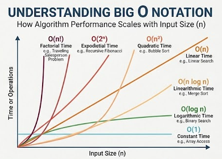
Big O notation measures how the resource requirements of an Algorithm—specifically running time and memory space—grow asymptotically as the input size ($N$) approaches infinity.

Instead of measuring execution in seconds or bytes (which change based on hardware), Big O focuses entirely on the growth rate of the operations relative to input growth.

Fundamental Mathematical Rules

When calculating Big O, you evaluate the total algebraic cost Function $T(N)$ and apply two mathematical simplifications:

1. Drop the Constants

As $N$ grows massive, small scaling factors become mathematically insignificant.

• Example: $T(N) = 3N + 5 \implies O(N)$
• Example: $T(N) = \frac{1}{2}N^2 \implies O(N^2)$

2. Drop the Non-Dominant Terms

Focus only on the single term that grows fastest.

• Example: $T(N) = N^2 + 5N + 100 \implies O(N^2)$
• Example: $T(N) = N\log N + N^3 \implies O(N^3)$

Step-by-Step Time Complexity Analysis

Strategy A: Iterative Loop Analysis

To analyze iterative algorithms, you map loops to algebraic equations by multiplying outer loops by inner loops.

Single Loops

Python

def print_items(n):
    for i in Range(n):
        print(i)  # Executes N times

• Analysis: The Basic print operation executes exactly $N$ times.
• Complexity: $O(N)$ (Linear Time)

Nested loops (Independent)

Python

def print_pairs(n):
    for i in Range(n):         # Runs N times
        for j in Range(n):     # Runs N times for every single outer Iteration
            print(i, j)

• Analysis: The total execution cost is $N \times N = N^2$.
• Complexity: $O(N^2)$ (Quadratic Time)

Nested loops (Dependent)

Python

def print_triangles(n):
    for i in Range(n):         # Runs N times
        for j in Range(i):     # Runs 0, then 1, then 2... up to N-1 times
            print(i, j)

• Analysis: This forms an arithmetic progression:$$0 + 1 + 2 + \dots + (N-1) = \frac{N(N-1)}{2} = \frac{N^2}{2} – \frac{N}{2}$$
• Applying Rules: Drop constants and non-dominant terms.
• Complexity: $O(N^2)$ (Quadratic Time)

Strategy B: Logarithmic Divergence (Divide and Conquer)

When an Algorithm cuts its remaining Data processing pool in half during each Iteration, it exhibits logarithmic scale growth.

Python

def binary_search(sorted_list, target):
    low = 0
    high = len(sorted_list) - 1
    
    while low <= high:
        mid = (low + high) // 2
        if sorted_list[mid] == target:
            return mid
        elif sorted_list[mid] < target:
            low = mid + 1
        else:
            high = mid - 1
    return -1

• Analysis: With each Array entry comparison, the remaining search window drops from $N \to \frac{N}{2} \to \frac{N}{4} \to \frac{N}{8}$.
• Calculation: How many times ($k$) can we divide $N$ by 2 before reaching 1?$$\frac{N}{2^k} = 1 \implies N = 2^k \implies k = \log_2 N$$
• Complexity: $O(\log N)$ (Logarithmic Time)

Strategy C: Recursive Call Trees

For recursive procedures, map out the branch Count per stack split and multiply it by the depth of the tree structure.

Python

def fibonacci(n):
    if n <= 1:
        return n
    return fibonacci(n - 1) + fibonacci(n - 2)

• Analysis: Every structural step down invokes two additional functions, doubling calls dynamically. The execution depth reaches a height of $N$.
• Calculation: Total branches = $2^0 + 2^1 + 2^2 + \dots + 2^N \approx 2^N$.
• Complexity: $O(2^N)$ (Exponential Time)

Step-by-Step Space Complexity Analysis

Space complexity tracks the additional maximum memory footprint allocated by an Algorithm during runtime, relative to input scale. It includes both Variables stored in memory heap space and active stacks frame states.

1. Auxiliary Allocation Space

Memory assigned directly for Variable manipulation arrays.

Python

def generate_lookup(n):
    arr = []
    for i in Range(n):
        arr.append(i * 2)  # Dynamically scales allocations up to N elements
    return arr

• Analysis: The Function allocates an Array holding $N$ distinct values inside memory.
• Complexity: $O(N)$ Space.

2. Call Stack Memory Space

Recursive algorithms take up execution Environment stack space, even if no explicit Variables are declared.

Python

def down_counter(n):
    if n <= 0:
        return
    down_counter(n - 1)  # Keeps frame Context open in execution stack

• Analysis: Before hitting the recursive base exit Condition ($n \le 0$), the compiler keeps all parental frames open in memory sequence. The stack depth holds exactly $N$ active frames simultaneously.
• Complexity: $O(N)$ Space.

Cheat Sheet: Standard Complexities Matrix

Big O Notation	Performance Class	Typical Paradigm Example
$O(1)$	Constant	Accessing an Array item by index; Hash map lookups.
$O(\log N)$	Logarithmic	Binary search operations; balanced tree navigation.
$O(N)$	Linear	Single pass tracking arrays; linear scans.
$O(N \log N)$	Linearithmic	Optimized sorting architectures (Merge Sort, Quick Sort).
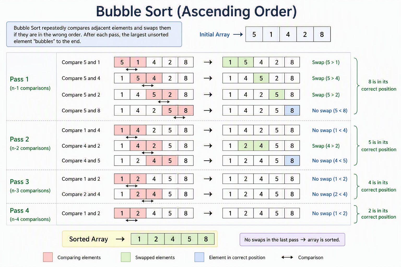
$O(N^2)$	Quadratic	Brute-force nested algorithms (Bubble Sort).
$O(2^N)$	Exponential	Exhaustive recursive calls without optimization.
$O(N!)$	Factorial	Generating all permutations of a set.

Guided Practice Case: Two-Sum Analysis

Let’s apply these steps to evaluate two distinct approaches to the classic “Two-Sum” problem.

Problem: Given an Array of integers nums and a target Integer target, return the indices of the two numbers that add up to target.

Method 1: The Brute Force Approach

Python

def two_sum_brute(nums, target):
    n = len(nums)
    for i in range(n):
        for j in range(i + 1, n):
            if nums[i] + nums[j] == target:
                return [i, j]
    return []

• Time Analysis: A nested Loop structures a dependent series execution: $(N-1) + (N-2) + \dots + 1$. Dropping non-dominant factors yields $O(N^2)$.
• Space Analysis: Only primitive pointers (i, j, n) are held in memory. Space does not scale based on Array size.
• Summary: Time: $O(N^2)$, Space: $O(1)$.

Method 2: The Hash Map Optimization

Python

def two_sum_optimized(nums, target):
    seen = {}  # Allocates hash map container
    for i, num in enumerate(nums):
        complement = target - num
        if complement in seen:
            return [seen[complement], i]
        seen[num] = i
    return []

• Time Analysis: We make a single pass through the Array Loop ($N$ items). Inside the Loop, checking if a value exists in a hash map takes constant time ($O(1)$). Total time scales linearly.
• Space Analysis: In the worst-Case scenario (no matching pairs exist), the seen hash map stores every single element from the input Array.
• Summary: Time: $O(N)$, Space: $O(N)$.

The Trade-Off Principle: Method 2 optimizes computational Time efficiency (moving from quadratic $O(N^2)$ down to linear $O(N)$) by deliberately investing more physical Space memory overhead ($O(1) \to O(N)$).